Building Neural Networks from Scratch

Brief summary

The objective from this page to understand how to implement a neural network from scratch without any external libraries, this page consider that you already have some knowledge of Artificial Neural Networks. The main reason for this is just to make more understandable the black box of Neural Networks. So, to this project, the main resource (but not the unique) is this video from Andrej Karpathy. I will cover how to implement AutoGrad for backpropagation. At the end of this post, you will cable of create MLPs without any external library.

Basic knowledge of derivative

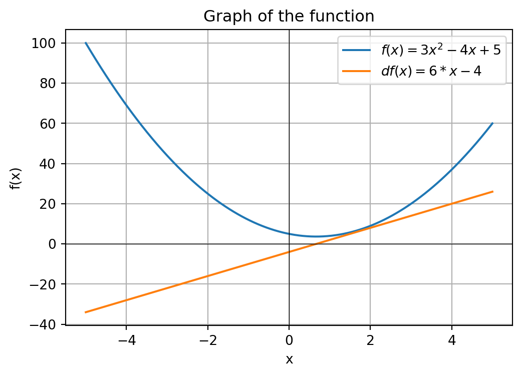
So, from the start, to make sense at how an NN train and learn something, you first need a very good understanding around the meaning of derivative operations. A derivative is an operation that gives us a formula that describes the slope of a function as it modifies a variable, but for out propose, we will only work with functions that generate linear derivatives. Thus, for the function \(f(x) = 3x^2 - 4x + 5\), see the graph below.

import numpy as np
import matplotlib.pyplot as plt

# Define the function
def f(x):
    return 3*x**2 - 4*x + 5

# Generate x values
x = np.linspace(-5, 5, 400)
y = f(x)

# Plot
plt.figure(figsize=(6, 4))
plt.plot(x, y, label=r"$f(x) = 3x^2 - 4x + 5$")
plt.axhline(0, color="black", linewidth=0.5)
plt.axvline(0, color="black", linewidth=0.5)
plt.xlabel("x")
plt.ylabel("f(x)")
plt.title("Graph of the function")
plt.legend()
plt.grid(True)
plt.show()

This function is easy to undestand and derivate analytic, the derivate is \(\frac{df(x)}{dx} = 6x - 4\). Plotting both function and his derivate, we get the graphic below.

import numpy as np
import matplotlib.pyplot as plt

# Define the function
def f(x):
    return 3*x**2 - 4*x + 5

def df(x):
    return 6*x - 4

# Generate x values
x = np.linspace(-5, 5, 400)
y = f(x)
y2 = df(x)

# Plot
plt.figure(figsize=(6, 4))
plt.plot(x, y, label=r"$f(x) = 3x^2 - 4x + 5$")
plt.plot(x, y2, label=r"$df(x) = 6*x - 4$")
plt.axhline(0, color="black", linewidth=0.5)
plt.axvline(0, color="black", linewidth=0.5)
plt.xlabel("x")
plt.ylabel("f(x)")
plt.title("Graph of the function")
plt.legend()
plt.grid(True)
plt.show()

The basic idea is that with we want to minimize the value of a function (main objective in deep learning), we just need to see the value of a derivative in some point A, that give us all the information we need to go to the minimum spot. Just do some numerical example, in the graph above, note that the minimum spot is in some value around 0 and 2, more close to 0 (precisely 2/3), so, just pick some random number, like -2, the value of \(f(x)\) with -2 is 25, and the derivative is -16. The number -16 represent the rate at which the function varies for each increase in the value of x at that point in specific. So, with we increase the value of X a little bit, we can lower the value of X, so probably, the \(f(-1.999)\) give us a lower value than \(f(-2)\)

def f(x):
    return 3*x**2 - 4*x + 5

print("f(-2)=",f(-2))
print("f(-1.999)=",f(-1.999))

f(-2)= 25
f(-1.999)= 24.984003

This is the general idea of how we can minimize some function, that is also the main idea of how gradient descendent works.

How to estimate gradients

In general, to make an framework for working with nn, its just an AutoGrad (a tool that can do differentiation automatically) and some fancy stuff for make more practical.

For start, lets make things the most simple for now. Our goal its make an class that can calc for us all the gradients (its the same as an derivative) from the function \(L = -2 \cdot \big((2 \cdot 3) + 10\big)\). But we don’t are comfortable derivate something with just numbers, so lets consider in this way the function:

a = 2
b = -3.0
c = 10
f = -2
e = a*b
d = e + c
L = d * f
L

-8.0

Just to make clear, the knowledge that we want with this, is ow much changes in the final result, increase the values of any of the variables a little To get the gradients, we can use an approximate that consists in adding a very small number \(h\) is all of the values, than subtract the new with the original, and divide by the \(h\). The code below shows how to do this with the variable \(a\):

a = 2
b = -3.0
c = 10
f = -2
e = a*b
d = e + c
L = d * f

h = 0.0001
a = 2 + h
b = -3.0
c = 10 
f = -2
e = a*b
d = e + c
L2 = d * f

print(f"L(2) = {L}")
print(f"L({a}) = {L2}")
print(f"The slope/gradient: {(L2 - L)/h}")

L(2) = -8.0
L(2.0001) = -7.999399999999998
The slope/gradient: 6.000000000021544

We will not use this method to create our autograd, but we can use this to verify with our gradients are right.

Lets making a simple AutoGrad

The basic idea of the AutoGrad we will make is make some very simple nodes, that represent the number in our calculation and will track all the last two nodes that make him. Basically, in \(L = -2 \cdot \big((2 \cdot 3) + 10\big)\), we will consider that a node can only save on number, like in the code representation

a = 2
b = -3.0
c = 10
f = -2
e = a*b
d = e + c
L = d * f

So, for start, lets make the basic of our class:

class Value:
    def __init__(self, data, _children=(), _op="", label=""):
        self.data = data
        self.grad = 0 # All nodes will start with no grad, becouse we dont know what is the grad (and for other math reaseon will explain soon)
        self._prev = set(_children) # Dont worry about this for know, we only use set for a little bit better performance
        self._op = _op # To save the operation, its usefull for debug
        self.label = label # You can ignore this, its just for the graphs I make below

    # This is just for us visualize our class
    def __repr__(self):
        return f"Value(data={self.data})"

So with this class, we can create some Value’s, but we cant use them for anything, so lets make some operations

class Value:
    def __init__(self, data, _children=(), _op="", label=""):
        self.data = data
        self.grad = 0
        self._prev = set(_children) 
        self._op = _op
        self.label = label # You can ignore this, its just for the graphs I make below

    # This is just for us visualize our class
    def __repr__(self):
        return f"Value(data={self.data})"


    def __add__(self, other):
        # We just add the data, and return a Value object with new data, and with pointes for the two number that make the out number
        out =  Value(self.data + other.data, (self,other), '+')
        return out
    
    def __mul__(self, other):
        out = Value(self.data * other.data, (self,other), "*")
        return out

And with this simples class, we can know calc our formula (not the gradients yet)

a = Value(2., label="a")
b = Value(-3.0, label="b")
c = Value(10., label="c")
f = Value(-2., label="f")
e = a * b; e.label="e"
d = e + c; d.label="d"
L = d * f; L.label="L"
L

Value(data=-8.0)

This calculation is known as pass forward Below, simply make a graph to visualize the operations (note that the operator is not a real node, but to visualize this it is better). The question is: how can we get the gradients for \(L\), \(d\) and \(f\)?

For \(L\), I think it´s a little obvious, its just 1, from calculus, the derivative for the function \(f(x) = x\) its 1. For \(d\) and \(f\), we it´s simple too, from calculus, de derivative \(f(x) = zx\) its just z, and this is the case for both \(d\) and \(f\). See the equation below \[ L(d,f) = d \cdot f \] \[ \frac{\partial L}{\partial d} = f \quad \text{and} \quad \frac{\partial L}{\partial f} = d \]

So, the gradient for \(d\) is the value of data in \(f\), and for the \(f\), it´s the value of data in \(d\), in this case, the grad of \(d\) is -2 and the grad of \(f\) is 4.

Now its start being interesting, we want to calc the gradient of \(e\) and \(c\) in relation of \(L\). From the chain of rule, we have the expression below: \[ \frac{\partial L}{\partial e} = \frac{\partial L}{\partial d} \cdot \frac{\partial d}{\partial e} \] Bascially, it´s saying that the gradient of \(e\) in relation with \(L\) it´s just the gradient of \(d\) in relation with \(L\) time \(e\) in relation with \(d\). This mean that we only have to calc the local gradient \(\frac{\partial d}{\partial e}\) because we already have calc the \(\frac{\partial L}{\partial d}\) and its save in d.grad. The same with \(c\) it´s true. So, from calculus, the gradient from an expression like \(f(x,y) = x + y\) its 1 for both \(x\) and \(y\). Thus, we have

\[ \frac{\partial d}{\partial e} = 1 \quad \text{and} \quad \frac{\partial d}{\partial c} = 1 \] \[ \frac{\partial L}{\partial e} = \frac{\partial L}{\partial d} \cdot \frac{\partial d}{\partial e} = -2 \cdot 1 = -2 \quad \text{and} \quad \frac{\partial L}{\partial e} = \frac{\partial L}{\partial d} \cdot \frac{\partial d}{\partial c} = -2 \cdot 1 = -2 \]

This is the strong concept that make the AutoGrad work, we only need to calc the local gradient and multiply with the gradient from the father of nodes (because the gradient of the father already is in relation with the last node).

So for the last two variables \(a\) and \(b\), its another multiplication, so the local grad of \(b\) its data of \(a\), and for \(a\) its data from \(b\). Put in a code, its just

L.grad = 1
d.grad = f.data
f.grad = d.data
e.grad = 1 * d.grad
c.grad = 1 * d.grad
a.grad = b.data * e.grad
b.grad = a.data * e.grad

This is a complete backward pass manual, know we need to make a code to this automatically for us

Automatically backward pass

To make this automatically, we probably notted that we need to start from the last node and go in a reverse order, this is necessery because for calc the gradient of and node, we need the local gradient of the variable, and the gradient of the father, the unique exception is the last node, because its gradient always will be 1. The way will we implement this, its just make a node do the calc of his childs gradients, lets see the mul function:

class Value:
    def __init__(self, data, _children=(), _op="", label=""):
        self.data = data
        self.grad = 0
        self._backward = None # Add this new parameter too save the func
        self._prev = set(_children) 
        self._op = _op
        self.label = label 

    def __mul__(self, other):
        out =  Value(self.data * other.data, (self,other), '+')
        
        def _backward():
            # We use += over =, because with we use the same node two times it will be reset, and with this node influences in two other nodes, its influence in final result, are the sum of the influence on both nodes
            self.grad += other.data * out.grad 
            other.grad += self.data * out.grad

        out._backward = _backward

        return out

Lets check with this can calc the gradients of \(d\) and \(f\)

a = Value(2., label="a")
b = Value(-3.0, label="b")
c = Value(10., label="c")
f = Value(-2., label="f")
e = a * b; e.label="e"
d = e + c; d.label="d"
L = d * f; L.label="L"

L.grad = 1

L._backward()
print("Grad of d:", d.grad)
print("Grad of f:", f.grad)

Grad of d: -2.0
Grad of f: 4.0

It works! So know, its just do for add too, below are the complete Value class

class Value:
    def __init__(self, data, _children=(), _op="", label=""):
        self.data = data
        self.grad = 0
        self._backward = lambda: None # Add this new parameter too save the func
        self._prev = set(_children) 
        self._op = _op
        self.label = label 

    def __mul__(self, other):
        out =  Value(self.data * other.data, (self,other), '+')
        
        def _backward():
            self.grad += other.data * out.grad 
            other.grad += self.data * out.grad

        out._backward = _backward

        return out

    # This is just for us visualize our class
    def __repr__(self):
        return f"Value(data={self.data})"


    def __add__(self, other):
        # We just add the data, and return a Value object with new data, and with pointes for the two number that make the out number
        out =  Value(self.data + other.data, (self,other), '+')
        def _backward():
            self.grad += out.grad 
            other.grad += out.grad

        out._backward = _backward

        return out

Lets check with we can calc all the gradients:

a = Value(2., label="a")
b = Value(-3.0, label="b")
c = Value(10., label="c")
f = Value(-2., label="f")
e = a * b; e.label="e"
d = e + c; d.label="d"
L = d * f; L.label="L"

L.grad = 1

L._backward() # Node L: Propagates gradient to d and f
d._backward() # Node d: Propagates gradient to e and c
f._backward() # Node f (Leaf): Does nothing (empty lambda)
e._backward() # Node e: Propagates gradient to a and b
c._backward() # Node c (Leaf): Does nothing
b._backward() # Node b (Leaf): Does nothing
a._backward() # Node a (Leaf): Does nothing

print(f"L data: {L.data}")
print("-" * 20)
print(f"Grad of L: {L.grad}") # Should be 1
print(f"Grad of f: {f.grad}") # Should be 4.0 (d.data)
print(f"Grad of d: {d.grad}") # Should be -2.0 (f.data)
print(f"Grad of c: {c.grad}") # Should be -2.0 (1 * d.grad)
print(f"Grad of e: {e.grad}") # Should be -2.0 (1 * d.grad)
print(f"Grad of b: {b.grad}") # Should be -4.0 (a.data * e.grad -> 2 * -2)
print(f"Grad of a: {a.grad}") # Should be 6.0 (b.data * e.grad -> -3 * -2)

L data: -8.0
--------------------
Grad of L: 1
Grad of f: 4.0
Grad of d: -2.0
Grad of c: -2.0
Grad of e: -2.0
Grad of b: -4.0
Grad of a: 6.0

It worked perfectly, know we only need to make a funcion that calls all _backward() in all nodes recursively. Therefore we will use an algorithm for generating the topological order of the graph. That is, a linear order in which we can execute the nodes without causing any kind of dependency problem. Explaining this algorithm in depth is outside the scope of this project, but it is not that complicated, see below:

# ... All methods of Value class
def backward(self):
    self.grad = 1
    # Montar ordem topologica
    topo = []
    visited = set()
    def build_topo(v):
        if v not in visited:
            visited.add(v)
            for child in v._prev:
                build_topo(child)
            topo.append(v)
    build_topo(self)

    for node in reversed(topo):
        node._backward()

Know, lets test our backward function

class Value:
    def __init__(self, data, _children=(), _op="", label=""):
        self.data = data
        self.grad = 0
        self._backward = lambda: None # Add this new parameter too save the func
        self._prev = set(_children) 
        self._op = _op
        self.label = label 

    def __mul__(self, other):
        out =  Value(self.data * other.data, (self,other), '+')
        
        def _backward():
            self.grad += other.data * out.grad 
            other.grad += self.data * out.grad

        out._backward = _backward

        return out

    # This is just for us visualize our class
    def __repr__(self):
        return f"Value(data={self.data})"


    def __add__(self, other):
        # We just add the data, and return a Value object with new data, and with pointes for the two number that make the out number
        out =  Value(self.data + other.data, (self,other), '+')
        def _backward():
            self.grad += out.grad 
            other.grad += out.grad

        out._backward = _backward

        return out

    def backward(self):
        self.grad = 1
        # create a topological order
        topo = []
        visited = set()
        def build_topo(v):
            if v not in visited:
                visited.add(v)
                for child in v._prev:
                    build_topo(child)
                topo.append(v)
        build_topo(self)

        for node in reversed(topo):
            node._backward()

a = Value(2., label="a")
b = Value(-3.0, label="b")
c = Value(10., label="c")
f = Value(-2., label="f")
e = a * b; e.label="e"
d = e + c; d.label="d"
L = d * f; L.label="L"


L.backward() 


print(f"L data: {L.data}")
print("-" * 20)
print(f"Grad of L: {L.grad}") # Should be 1
print(f"Grad of f: {f.grad}") # Should be 4.0 (d.data)
print(f"Grad of d: {d.grad}") # Should be -2.0 (f.data)
print(f"Grad of c: {c.grad}") # Should be -2.0 (1 * d.grad)
print(f"Grad of e: {e.grad}") # Should be -2.0 (1 * d.grad)
print(f"Grad of b: {b.grad}") # Should be -4.0 (a.data * e.grad -> 2 * -2)
print(f"Grad of a: {a.grad}") # Should be 6.0 (b.data * e.grad -> -3 * -2)

L data: -8.0
--------------------
Grad of L: 1
Grad of f: 4.0
Grad of d: -2.0
Grad of c: -2.0
Grad of e: -2.0
Grad of b: -4.0
Grad of a: 6.0

It´s worked perfectly again, know we already have a functional AutoGrad system, know, it´s just need to add more operations and we will be capable of create our propely framework of Deep Learning using our own AutoGrad. Before going to the next part, see the code bellow, its the same that we create together, but with some little changes, try to figure out what they’re for (Hint, they’re important for the next part)

class Value:
    def __init__(self, data, _children=(), _op="", label=""):
        self.data = data
        self.grad = 0
        self._backward = lambda: None 
        self._prev = set(_children) 
        self._op = _op
        self.label = label 

    def __mul__(self, other):
        other = other if isinstance(other, Value) else Value(other)
        out =  Value(self.data * other.data, (self,other), '+')
        
        def _backward():
            self.grad += other.data * out.grad 
            other.grad += self.data * out.grad

        out._backward = _backward

        return out

    def __repr__(self):
        return f"Value(data={self.data})"


    def __add__(self, other):
        other = other if isinstance(other, Value) else Value(other)
        out =  Value(self.data + other.data, (self,other), '+')
        def _backward():
            self.grad += out.grad 
            other.grad += out.grad

        out._backward = _backward

        return out
    
    def __pow__(self, other):
        assert isinstance(other, (int, float)), "only supporting int/float powers for now"
        out = Value(self.data**other, (self,), f'**{other}')

        def _backward():
            self.grad += (other * self.data**(other-1)) * out.grad
        out._backward = _backward

        return out

    def __neg__(self): 
        return self * -1

    def __sub__(self, other): 
        return self + (-other)

    def __radd__(self, other): 
        return self + other

    def backward(self):
        self.grad = 1
        # create a topological order
        topo = []
        visited = set()
        def build_topo(v):
            if v not in visited:
                visited.add(v)
                for child in v._prev:
                    build_topo(child)
                topo.append(v)
        build_topo(self)

        for node in reversed(topo):
            node._backward()

Lets make our Deep Learning framework

Building a Neuron

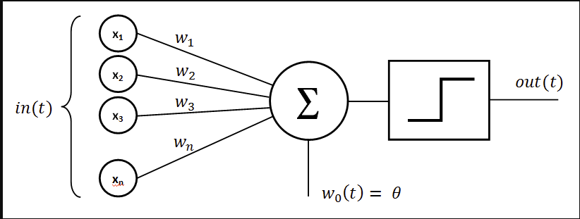
So, for now, we have already created our own engine to calculate our gradients. Thus, lets start making a simple artificial neuron. If you don’t know or don’t remember how a neuron work, basically it receives inputs, multiply each one by some weight, sum all values, and last, pass this value in a non-linear function

Figure 1: An Artificial Neuron

To start, we can make a simple class for our neuron:

import random
class Neuron:
    def __init__(self, input_num, non_linear=True):
        self.w = [Value(random.uniform(-1,1)) for _ in range(input_num)] # This basicaly creates a list of Value's from a uniform distribuition with lenth equals to input_num
        self.b = Value(random.uniform(-1,1)) # This is for the bias, explain deeply the importance of this is out of scope, but you can think bias its just a special weight that dosnt multiply the inputs, just sum in the sum part.

    # Call is a special function in python, its like __add__, the sintax for use this is when you just put () after the object, like range(x)
    def __call__(self,x):
        out = sum((wi*xi for wi,xi in zip(self.w, x)), self.b) # This just do the calculation of a neuron until the sum part
        return out
    
    def parameters(self):
        return self.w + [self.b] # this function just return all the parameters of our neuron

And, its just it, a completely and functional artificial neuron.

Know, lets test if this are working

n = Neuron(2)
x = [2, 3, 4]
out = n(x)
print(out, n.parameters())

Value(data=2.7606105336395843) [Value(data=0.34610789511609674), Value(data=0.8252449036669098), Value(data=-0.4073399675933387)]

Works, lets move on.

Building a Layer

So, we already create an simple Neuron, now, we just need to line them up for make a Layer.

class Layer:
    def __init__(self, input_num, output_num, non_linear=True):
        self.neurons = [Neuron(input_num) for _ in range(output_num)] # Create a list of neurons that accept input_num variables in input, and will generate output_num outputs
        self.non_linear = non_linear

    # Just process all operations in all neurons with the input
    def __call__(self,x):
        outs = [n(x) for n in self.neurons]

        if self.non_linear:
            outs = [out.tahn() for out in outs]

        return outs[0] if len(outs) == 1 else outs
    
    def parameters(self):
        out = []
        for neuron in self.neurons:
            out.extend(neuron.parameters()) # Add the values in an unique list
        return out

For this Layer class, we need to implement the tahn (tangent hyperbolic) function. It’s formula is: \[ \tanh(x) = \frac{e^x - e^{-x}}{e^x + e^{-x}} \]

Note that there is 3 operations that we don’t implement to make this, so, lets implement them. For know, I presume that you understand how to implement this, so, try your self, you can search in google for this, just don’t use an llm.

import math
# Its not really necessary to add exp, subtraction or divided, but its good with you do 😊
def tahn(self):
    x = self.data
    t = (math.exp(x) - math.exp(-x))/ (math.exp(x) + math.exp(-x))
    out = Value(t, (self,), "tahn")

    # We can derivate, or just pick up on google
    def _backwards():
        self.grad += (1 - t**2) * out.grad
    
    out._backward = _backward
    return out

Let’s test if this work

x = [2, 3, 4]

layer = Layer(3,3)
layer(x), layer.parameters()

([Value(data=0.9996646615551876),
  Value(data=0.9999791585105655),
  Value(data=-0.9747811998177511)],
 [Value(data=-0.2399760854356343),
  Value(data=0.5672209838656024),
  Value(data=0.6526425611040982),
  Value(data=0.5143938500523895),
  Value(data=0.7498233764763123),
  Value(data=-0.20504799838269894),
  Value(data=0.9718665298515214),
  Value(data=0.9638819394987441),
  Value(data=-0.9427159532454912),
  Value(data=-0.5007685680188607),
  Value(data=0.19206424478156947),
  Value(data=0.4391690659468055)])

Work well, this is pretty simple too. Now let’s move to the last part, create an complete Artificial Neural Network

Building an MLP

For last, we will create a Multilayer Perceptron, for this, we just need to to line layer up.

class MLP:
    def __init__(self, input_num, outputs_nums):
        self.layers = []
        values = [input_num] + outputs_nums
        for id in range(len(outputs_nums)-1): # This work for create an unique list used to describe input and output for all layers
            self.layers.append(Layer(values[id], values[id+1]))
        self.layers.append(Layer(values[-2], values[-1], non_linear=False))

    def __call__(self, X):
        for layer in self.layers: # This works because with exception from the first, each layer just receive the input from the last layer
            X = layer(X)
        return X

    def parameters(self):
        out = []
        for layer in self.layers:
            out.extend(layer.parameters())
        return out

And, its finish, just need to test now

nn = MLP(3, [6,6,1])
x = [2, 3, 4]

nn(x) # You can test the parameters

Value(data=-0.7919551271747531)

Training our neural network

In the last part, we create a MLP, but we don’t fit them in any data. Lets create a function and values with some noise

import random

def f(x,y,z):
    return 0.04*x**2 + 0.07*y*x - z + random.gauss(0, 1)/5

X = []
y = []
for i in range(100):
    X.append([random.uniform(-5,5) for _ in range(3)])
    y.append(f(X[i][0],X[i][1],X[i][2]))

To implement the train loop, we will need one more thing, there is an loss functions, this is just an metric that describes how well our model are fitting in data. For these case, we will use Mean Squared Error, so the steps for the training loop, its, calc the prediction, calc the loss, calc the gradients, subtract the gradients from the weights, reset the gradients values (our code accumulate the gradients) and do it again, and again.

ann = MLP(3, [8, 8, 1]) 
 
for i in range(50): # Our code will do 50 epochs of training 
    y_pred = [ann(x) for x in X] # Our model only accept one prediction per time
    loss = sum((pred-origin)**2 for pred,origin in zip(y_pred, y)) 

    loss.backward() # Calc of gradients 

    for p in ann.parameters():
        p.data = p.data - 0.001*p.grad # Updating weights, we multiply the gradient by a small number called learning rate, we do this for not have problems with model convergence
        p.grad = 0
    print(f"Epoch {i}, Loss: {loss}")

Epoch 0, Loss: Value(data=1173.927825101448)
Epoch 1, Loss: Value(data=479.3293651535565)
Epoch 2, Loss: Value(data=274.5878032027161)
Epoch 3, Loss: Value(data=179.24830078948708)
Epoch 4, Loss: Value(data=145.57014093033285)
Epoch 5, Loss: Value(data=135.2468547794671)
Epoch 6, Loss: Value(data=128.96468805258488)
Epoch 7, Loss: Value(data=123.73377230062457)
Epoch 8, Loss: Value(data=119.24956713114472)
Epoch 9, Loss: Value(data=115.34916728015705)
Epoch 10, Loss: Value(data=111.9069266409732)
Epoch 11, Loss: Value(data=108.81655285791855)
Epoch 12, Loss: Value(data=105.98954851293747)
Epoch 13, Loss: Value(data=103.35366087728872)
Epoch 14, Loss: Value(data=100.85140836678144)
Epoch 15, Loss: Value(data=98.43793989880551)
Epoch 16, Loss: Value(data=96.07888048817817)
Epoch 17, Loss: Value(data=93.7488216361225)
Epoch 18, Loss: Value(data=91.43017742079934)
Epoch 19, Loss: Value(data=89.11255823869828)
Epoch 20, Loss: Value(data=86.79210670629311)
Epoch 21, Loss: Value(data=84.4706497341805)
Epoch 22, Loss: Value(data=82.15431043581388)
Epoch 23, Loss: Value(data=79.8516216415455)
Epoch 24, Loss: Value(data=77.57130376585995)
Epoch 25, Loss: Value(data=75.32018414386577)
Epoch 26, Loss: Value(data=73.10179409190116)
Epoch 27, Loss: Value(data=70.91631914225951)
Epoch 28, Loss: Value(data=68.76231336621191)
Epoch 29, Loss: Value(data=66.64041601255104)
Epoch 30, Loss: Value(data=64.55760585859981)
Epoch 31, Loss: Value(data=62.52884802189379)
Epoch 32, Loss: Value(data=60.57154326368767)
Epoch 33, Loss: Value(data=58.6963545301056)
Epoch 34, Loss: Value(data=56.903006792033935)
Epoch 35, Loss: Value(data=55.185875697576535)
Epoch 36, Loss: Value(data=53.541247825483175)
Epoch 37, Loss: Value(data=51.98022532924802)
Epoch 38, Loss: Value(data=50.57101858010987)
Epoch 39, Loss: Value(data=49.60115194381445)
Epoch 40, Loss: Value(data=50.452864150600426)
Epoch 41, Loss: Value(data=58.13598315203789)
Epoch 42, Loss: Value(data=99.44026776624415)
Epoch 43, Loss: Value(data=173.6608093660121)
Epoch 44, Loss: Value(data=290.50097477153923)
Epoch 45, Loss: Value(data=111.89952934255297)
Epoch 46, Loss: Value(data=67.26368862356497)
Epoch 47, Loss: Value(data=55.093670302415795)
Epoch 48, Loss: Value(data=49.50636689868851)
Epoch 49, Loss: Value(data=46.54826277713668)

Work, but not very well, it’s possible to improve this changing the activation function by an ReLU. But for our propose, it’s good enough. Lets just see the values coming from our model

y_pred = ann(X[1])
print(f"Real value: {y[1]}\nPredict value: {y_pred}") 

Real value: 3.561263195532192
Predict value: Value(data=3.0152658379527537)